
Direct Numerical Simulation of Boundary Layer Transition to Turbulence in a Hypersonic Wind Tunnel
JAXA Supercomputer System Annual Report February 2024-January 2025
Report Number: R24EFHC0309
Subject Category: Common Business
- Responsible Representative: Naoyuki Fujita, Security and Information Systems Department, Supercomputer Division
- Contact Information: Shingo Matsuyama(matsuyama.shingo@jaxa.jp)
- Members: Shingo Matsuyama
Abstract
In experiments of boundary layer turbulence transitions by hypersonic wind tunnels, it is known that the first source of disturbance that causes boundary layer transitions on the wind tunnel model is noise (e.g., pressure disturbances) radiated by the turbulent boundary layer that develops on the wind tunnel nozzle wall. The objective of this study is to reproduce the turbulent transition of the boundary layer on the nozzle wall and on the model wall in a hypersonic wind tunnel by Direct Numerical Simulation (DNS). In actual hypersonic wind tunnel tests, turbulent transitions are measured without understanding the effects of noise in the freestream, but the DNS conducted in this study enables us to understand how the noise generated by the turbulent boundary layer on the nozzle wall affects the turbulent boundary layer transitions on the wind tunnel model. This information is indispensable for improving the measurement of boundary layer transitions in hypersonic wind tunnels. In addition, the prediction of turbulent transition is an important issue in terms of drag and heating increase for hypersonic aircraft, which are expected to be developed by private companies in the future. The turbulent transition data obtained in this study will also provide important knowledge for understanding the boundary layer transition on the hypersonic aircraft due to atmospheric disturbances.
Reference URL
N/A
Reasons and benefits of using JAXA Supercomputer System
In order to analyze the turbulent transition process in the boundary layer of a hypersonic wind tunnel nozzle using DNS, it is necessary to resolve turbulence up to near the Kolmogorov scale. Therefore, for high Reynolds number flows where turbulent transitions occur, the grid size will be much larger than one billion points. The computational cost of such a large-scale three-dimensional unsteady analysis is extremely high and can only be achieved using a supercomputer.
Achievements of the Year
1. Summary of Results
In this study, DNS was conducted for the turbulent transition process in the boundary layer that occurs in a hypersonic wind tunnel, with the aim of achieving an initial disturbance that accurately simulates reality. As the results of this year's study, we first report the results of DNS that reproduced the freestream disturbance in the hypersonic wind tunnel. The DNS, which simulates a hypersonic wind tunnel nozzle, generates a turbulent boundary layer on the nozzle wall and reproduces the freestream disturbance caused by the noise radiated by the turbulent boundary layer. Another result was a DNS analysis of two flat plates placed facing each other to simulate the arrangement of the wind tunnel nozzle and the measurement model. In this analysis, an artificial disturbance was added to one of the two plates (corresponding to the nozzle wall) to generate a turbulent boundary layer, and the noise radiated by the turbulent boundary layer caused a boundary layer transition on the other plate (corresponding to the measurement model).
2. Numerical Method
In this study, DNS was conducted using the thermochemical nonequilibrium flow analysis code JONATHAN, which has been developed and maintained by the Aviation Technology Directorate (ATD) of JAXA. The three-dimensional compressible Navier-Stokes equations were used as governing equations for the flow field, and conservation equations for density, momentum, and energy were solved assuming a frozen flow without chemical reaction. The governing equations were discretized using a finite volume approach, and the convective flux was calculated using the SLAU2 scheme. For higher spatial accuracy, the scalar quantities of density and pressure were interpolated by the second-order MUSCL method, and the velocity components were interpolated by a fifth-order polynomial without limiter. For time integration, a two-stage second-order Runge-Kutta method was used.
3. Results
3.1 Reproduction of Freestream Disturbance in a Hypersonic Wind Tunnel by DNS
DNS of turbulent boundary layer was performed for the Mach 7 nozzle geometry of the 0.5 m/1.27 m hypersonic wind tunnel installed at the ATD of JAXA. Z-direction was taken as flow direction (nozzle axis direction) and z = 0 was taken as nozzle throat position. The DNS analysis was performed in two different ways, solving only for the 1/2 (180 degrees) and 1/4 (90 degrees) part of the circumferential direction in the region downstream of the throat (z > 0.5 m). The total number of computational cells used for each DNS analysis was approximately 5.72 billion and 2.86 billion, respectively.
First, the laminar nozzle flow was formed by conducting analysis for approximately 3 ms from an initial state of completely stationary flow. Then, a disturbance was applied inside the boundary layer at z = 0.6 m to cause a turbulent transition in the boundary layer on the nozzle wall, and further analysis was performed for approximately 12 ms.
The instantaneous flow field at t=15 ms obtained by the DNS analysis, in which a 1/2 (180 degrees) part was solved in the circumferential direction, is shown in Figure 1. To visualize the noise radiated by the turbulent boundary layer, a pseudo-Schlieren image was created by the density gradient distribution. The instantaneous flow field in the y-z cross section (x=0 m) shows the boundary layer transition to turbulence around z = 0.8 m. The pseudo-Schlieren image also visualizes the noise radiated by the turbulent boundary layer. The strong noise associated with the turbulent transition propagates toward the center of the nozzle at the beginning of the transition at z = 0.8m. Further downstream, the noise structure becomes finer as the turbulent boundary layer develops and propagates toward the center of the nozzle at an angle of about 25 degrees to the flow direction. The instantaneous flow field in the x-y cross section at z = 3 m near the nozzle exit (z = 3.258 m) shows a well-developed turbulent boundary layer. As the pseudo-Schlieren image of the x-y cross section shows, the noise due to the turbulent boundary layer does not form large concentric structures but rather propagates and converges toward the nozzle center as fine, fragmented waves.
To evaluate the effect of computational domain size in the nozzle circumferential direction, the results of a DNS analysis in which only a 1/4 (90 degrees) part was solved are shown in Figure 2 (displayed by animation). The effect of the smaller circumferential computational domain is insignificant, and the transition position of the boundary layer and the noise radiated by the turbulent boundary layer are similar to the results with the 1/2 (180 degrees) computational domain.
The present analysis successfully reproduced the freestream disturbance in a hypersonic wind tunnel by DNS. Although it is necessary to validate the DNS in the future by acquiring freestream noise spectra through wind tunnel tests, the data obtained by the DNS analysis is expected to be used for modeling freestream disturbance.
3.2 DNS of Boundary Layer Transition to Turbulence between Two Flat Plates Placed Facing Each Other
As mentioned above, in a hypersonic wind tunnel test, noise radiated from the turbulent boundary layer developed on the nozzle wall causes freestream disturbance, and the turbulent transition of the boundary layer occurs on a model set up in the wind tunnel by the freestream noise as an initial disturbance. To simulate such an arrangement of the wind tunnel nozzle wall and the model, a DNS analysis was performed on two flat plates placed facing each other. The leading edge of the flat plate was set to x = y = 0 with the x, y, and z directions as the flow direction, wall vertical direction, and span direction, respectively, with another flat plate offset downstream by 2.7 m and vertically by 0.2 m. The total number of computed grid points for this analysis is approximately 1.06 billion. In this DNS analysis, a turbulent boundary layer is first generated by adding disturbances inside the boundary layer on the flat plate placed on the lower side. No artificial disturbance was added to the boundary layer on the upper flat plate to investigate whether transitions also occur on the upper flat plate due to noise radiated by the turbulent boundary layer developing on the lower flat plate.
The results of the DNS analysis are shown in Figures 3 and 4 (displayed by animation). As with the DNS of the wind tunnel nozzle, a pseudo-Schlieren image was created by the density gradient. The results in the figures are scaled up by a factor of 5 in the y direction to facilitate visibility of the boundary layer. First, it can be confirmed that on the flat plate placed on the lower side, the boundary layer transitions to completely turbulent flow at around x = 0.4 m by adding a disturbance. In addition, acoustic noise is radiated from the edge of the turbulent boundary layer in the downstream direction, obliquely upward to the right. The noise emitted from the turbulent boundary layer on the lower flat plate passes through the oblique shock wave formed at the leading edge of the upper flat plate and enters the boundary layer. On the upper flat plate, the incident noise acts as an initial disturbance and makes a transition to turbulence at about 0.3 m from the leading edge of the plate.
In the present DNS analysis, we attempted to reproduce a turbulent transition process similar to that of a real wind tunnel test by generating a disturbance from outside the boundary layer in the DNS of the boundary layer transition. Two flat plates were placed facing each other, and a turbulent boundary layer was generated by an artificial disturbance on the lower plate, and the noise radiated by the turbulent boundary layer caused the boundary layer to transition to turbulence on the upper plate as well. The transition on the upper flat plate is considered to be quite similar to that observed in actual hypersonic wind tunnel tests (turbulent transition of the boundary layer on the measurement model due to the freestream noise). The results of the present DNS analysis are expected to improve our understanding of the turbulent transition processes that occur in actual wind tunnel tests.
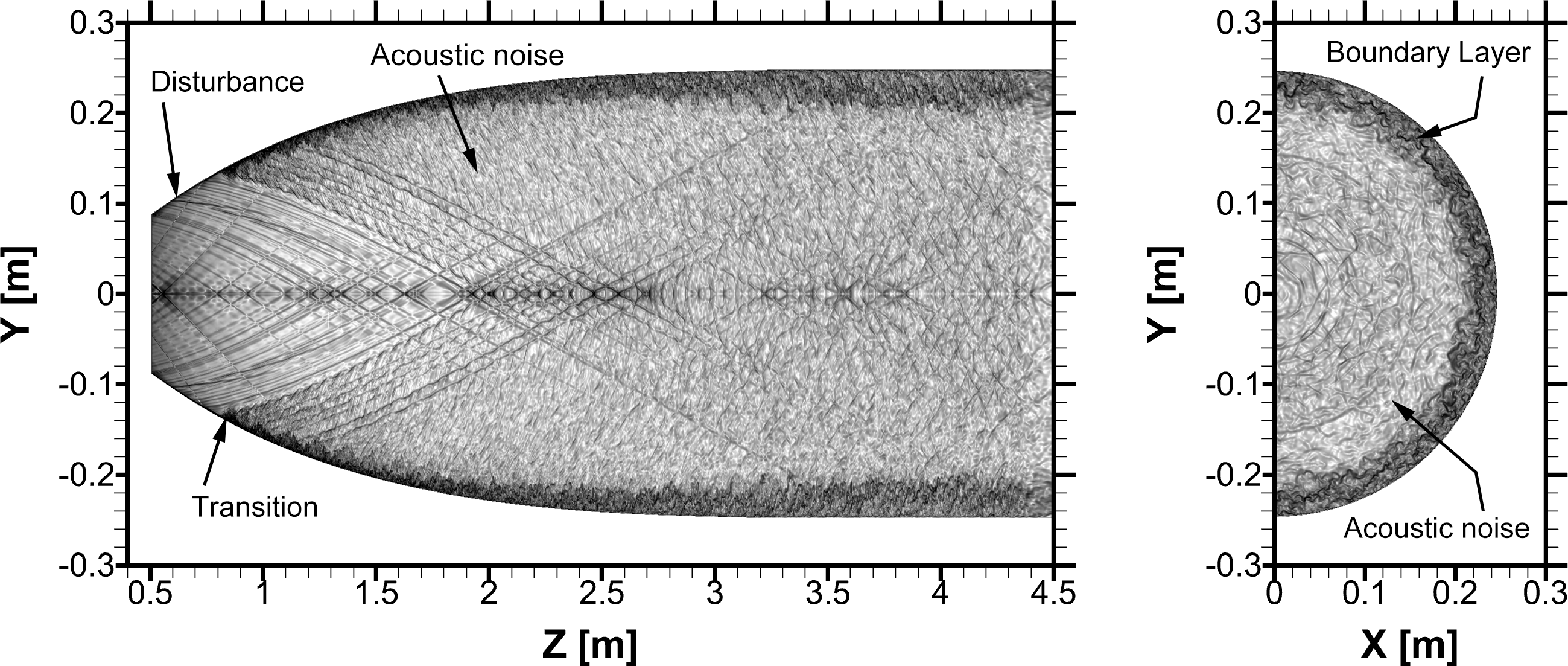
Fig.1: Instantaneous flow field at t=15 ms obtained by DNS analysis of a hypersonic wind tunnel nozzle. Pseudo-Schlieren image created by density gradient from DNS results solved for the 1/2 (180 degrees) part of the nozzle circumferential direction.
Fig.2(video): Result of DNS analysis solving only the 1/4 (90 degrees) part of the nozzle circumferential direction.
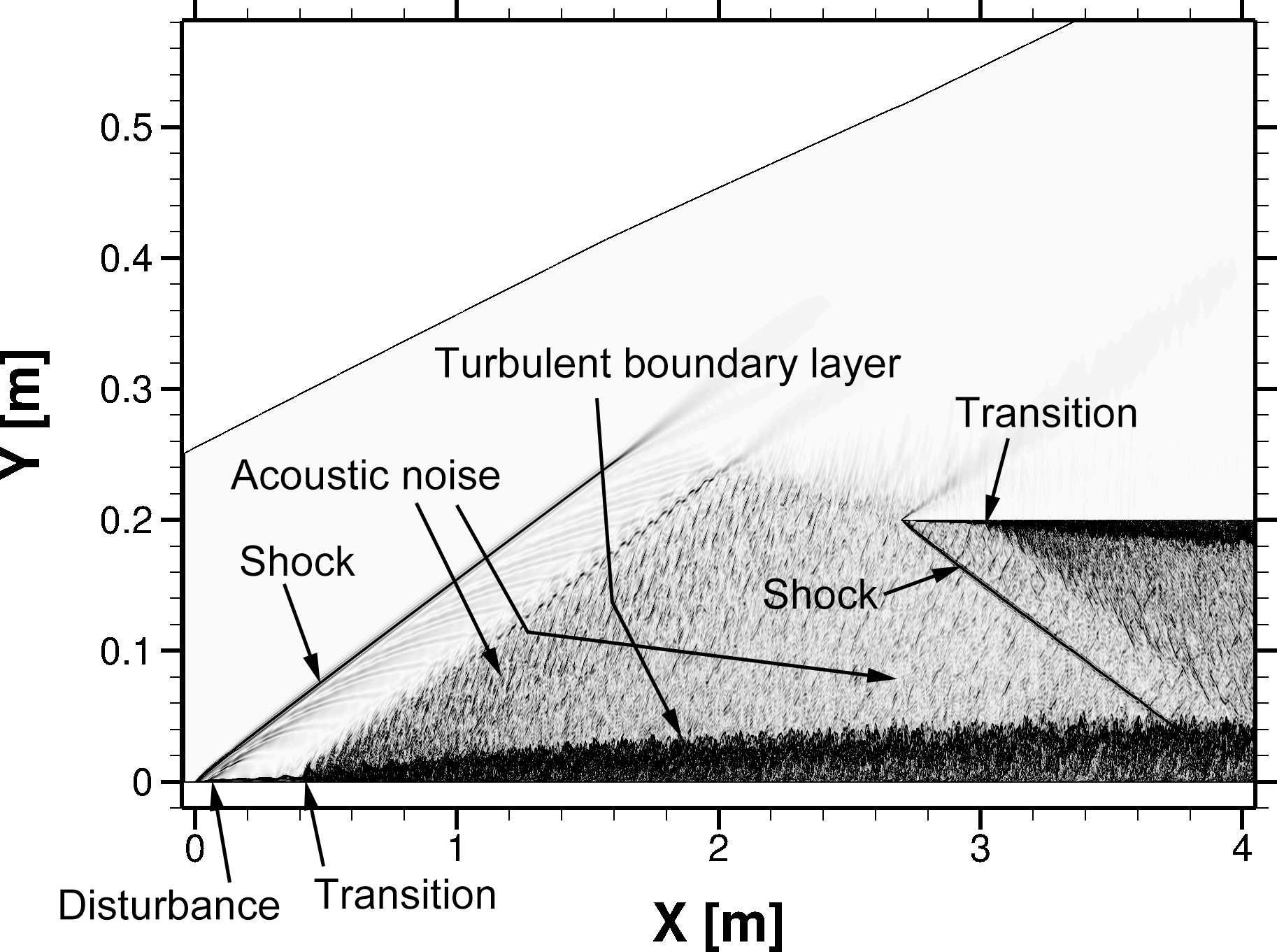
Fig.3: Results of DNS analysis for two flat plates placed facing each other. The instantaneous flow field is shown in a pseudo-Schlieren image created by density gradient.
Fig.4(video): Results of DNS analysis for two flat plates placed facing each other. The boundary layer transition process is shown by animation using a pseudo-Schlieren image.
Publications
- Non peer-reviewed papers
1) Shingo Matsuyama, "Some Attempts to Bridge the Gap Between DNS and Wind Tunnel Testing of Hypersonic Boundary Layer Transition," Journal of the Visualization Society of Japan, Volume 45, Issue 172, pp.3-6, 2025.
- Oral Presentations
1) Shingo Matsuyama, "DNS Analysis of Freestream Disturbances in a Hypersonic Wind Tunnel," the 55th JSASS Annual Meeting, 2024.
2) Shingo Matsuyama, Yuki Ide, Keisuke Fujii, "DNS of Hypersonic Boundary Layer Transition Solving the Whole Wind Tunnel Nozzle and Model," Symposium on Flight Mechanics and Astrodynamics: 2024.
3) Shingo Matsuyama, "Some Considerations for Performing High-Fidelity DNS of Boundary Layer Transitions Encountered During Actual Atmospheric Entries," Symposium on Flight Mechanics and Astrodynamics: 2024.
Usage of JSS
Computational Information
- Process Parallelization Methods: MPI
- Thread Parallelization Methods: OpenMP
- Number of Processes: 16340 - 32680
- Elapsed Time per Case: 120 Hour(s)
JSS3 Resources Used
Fraction of Usage in Total Resources*1(%): 0.00
Details
Please refer to System Configuration of JSS3 for the system configuration and major specifications of JSS3.
| System Name | CPU Resources Used(Core x Hours) | Fraction of Usage*2(%) |
|---|---|---|
| TOKI-SORA | 0.00 | 0.00 |
| TOKI-ST | 0.00 | 0.00 |
| TOKI-GP | 0.00 | 0.00 |
| TOKI-XM | 0.00 | 0.00 |
| TOKI-LM | 0.00 | 0.00 |
| TOKI-TST | 0.00 | 0.00 |
| TOKI-TGP | 0.00 | 0.00 |
| TOKI-TLM | 0.00 | 0.00 |
| File System Name | Storage Assigned(GiB) | Fraction of Usage*2(%) |
|---|---|---|
| /home | 24.50 | 0.02 |
| /data and /data2 | 1531.00 | 0.01 |
| /ssd | 251.00 | 0.01 |
| Archiver Name | Storage Used(TiB) | Fraction of Usage*2(%) |
|---|---|---|
| J-SPACE | 2.76 | 0.01 |
*1: Fraction of Usage in Total Resources: Weighted average of three resource types (Computing, File System, and Archiver).
*2: Fraction of Usage:Percentage of usage relative to each resource used in one year.
ISV Software Licenses Used
| ISV Software Licenses Used(Hours) | Fraction of Usage*2(%) | |
|---|---|---|
| ISV Software Licenses(Total) | 0.00 | 0.00 |
*2: Fraction of Usage:Percentage of usage relative to each resource used in one year.
JAXA Supercomputer System Annual Report February 2024-January 2025